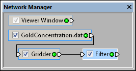
Select the Filter module in the Network Manager
to display its properties in the Property Manager.

Use the Filter module to choose one of many
filter types to apply to the input lattice.
The Network | Computational | Filter command adds a Filter module.
The Filter module applies a digital filter to a uniform lattice. The lattice may be two-dimensional (images) or three-dimensional (volumes). Each filter reads the input lattice, performs a particular filtering operation on the data values in the lattice nodes, and sends the results to the output lattice. The input and output lattices are always the same size and type.
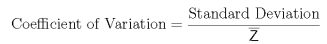
Filter module computations include data statistics such as local minimum, maximum, median, average, standard deviation; and image modification such as brightness and contrast.
Uniform lattice is the input type for the Filter module.
The Filter module may be connected to the Graphics Output Modules or the Computational Modules. An Info Module may also be connected to the output node.
The Filter properties are described below.
Select the Filter module in the Network Manager
to display its properties in the Property Manager.
Use the Filter module to choose one of many
filter types to apply to the input lattice.
The Input property shows the source to which the module is connected. This option cannot be changed in the Property Manager, but can be changed in the Network Manager by changing the module input.
The Filter type is the type of filter to apply to the input lattice. There are six categories of filters: Linear Convolution; Nonlinear - Order Statistics; Nonlinear - Moment Statistics; Nonlinear - Other; Nonlinear - Edge Detection; and Nodal. To change the filter type, click on the existing option and select the desired option from the list.
All of the filters are space-domain filters (currently, there are no frequency-domain filters). Note: This filter is applied to ALL components. Use the Subset module to apply filtering to individual components.
Use the Orientation option to specify the orientation of the filter. The first three choices— XY planes, XZ planes, and YZ planes— orient the filter in the specified direction and apply it to all slices of the lattice. The 3D option applies a full three-dimensional filter. Note: when this module is connected to a two-dimensional lattice, the three-dimensional orientation is disabled and this choice defaults to the two-dimensional lattice orientation. To change the orientation, click on the existing option and select the desired option from the list.
The Kernal size is the the size of the convolution kernel. The kernel is centered on the node being filtered and defines the neighborhood of surrounding nodes used to calculate the center node. If the kernel size is N, then the filtering kernel is NxNxN nodes in three dimensions. Not all filters use a convolution kernel, and for these the kernel size property is hidden. Kernel sizes must be odd to maintain symmetry. To change the Kernal size, highlight the existing value and type a new value or click the  button to increase or decrease the neighborhood size.
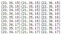
The neighborhood of an output lattice node is a cubic sub- array of nodes in the input lattice that is centered on the corresponding input lattice node. It has three equal dimensions, known as the kernel size. It must be noted that this concept of a neighborhood does not disallow that application of a lattice filter to a two-dimensional lattice. In the case of a two-dimensional lattice, one of the three dimensions is simply equal to 1. Since the neighborhood is centered on a node, the width, height, and depth must all be odd numbers. For example, if the kernel size is 3, the neighborhood of the output lattice node at (21, 31, 16) is the following rectangular sub-array of 27 input lattice nodes:
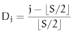
If kernel size of the neighborhood is represented by S, then the number of nodes in the neighborhood equals SxSxS. Furthermore, the nodes in the neighborhood of node (a,b,c) can be enumerated as 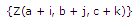 where
where
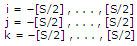
where [S/2] represents the largest integer less than or equal to S/2.
Click the  next to the Input Components to open the components list. Check the box next to the Component to pass the checked component through the filter. Unchecked components pass through the filter unaltered (unfiltered). This option allows the alpha channel of RGBA images to be excluded since this is not usually desired.
Click the next to the Edge Handling to open the options for handling data near the edge of the lattice.
Use the Edge handling option to specify how to handle edge effects when the kernel overhangs the edge of the lattice. Many filters, e.g., convolution filters, require a neighborhood of data around the lattice node being filtered. When filtering nodes along the edge, the neighborhood is incomplete on one or more sides. To change the edge handling, click on the existing option and select the desired option from the list. These options specify how to handle this condition:
Blank - Any lattice node with a neighborhood that overlaps more than one edge is blanked. For example, if the neighborhood size is 3x3x3, then every application of the filter blanks one plane (sheet) of nodes on each lattice face. Every application of the filter shrinks the active lattice by 2 rows, 2 columns, and 2 planes. Similarly, a 5x5x5 filter neighborhood blanks 4 rows, 4 columns, and 4 planes.
Ignore - Only the available neighborhood is used; calculations involving off-lattice nodes are ignored.
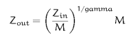
Replicate - Voxels at the edge of the input lattice are replicated. For example, consider a lattice with  rows,
rows,  columns, and
  planes. If the specified coordinate
  is off the edge of the lattice, the rules are
  where
where 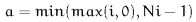 ,
, 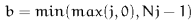 , and
, and 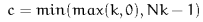 .
.
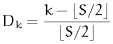
Mirror - Set off-lattice nodes to the symmetrically reflected node on the other side of the node being filtered; that is, treat the out-of-range coordinates as a mirror (reverse) of the corresponding in-range coordinates. Consider a lattice with rows, columns, and planes. If the specified coordinate (a,b,c) is off the edge of the lattice, the rules are where
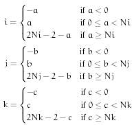
Cyclic wrap - Set off-lattice nodes by wrapping around to the opposite side of the lattice in three dimensions. If you go off the lattice on the right face, you come back on the left; if you go off the top, you come back on the bottom. This method is consistent with Fourier analysis which does this implicitly. For a lattice with rows, columns, and planes, the rules are where
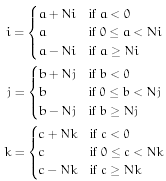
Fill - Fill beyond the edge with a user-specified constant. A common value for the fill is the arithmetic average of the lattice. This is the default method. For a lattice with rows, columns, and planes, the rules are 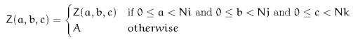 where
where  is the user-specified constant.
When the Edge handling is set to Fill, the Edge fill option becomes available. This is the value used to apply to the edge of the lattice. To change the value, highlight the existing value and type the desired value.
Click the next to the Blank Handling to open the options for handling blanked nodes in the lattice.
Use the Blank handling option to determine how to handle blanked nodes within the lattice. To change the way blank values are handled, click on the existing option and select the desired option from the list. Options include:
Expanded - Blanked nodes and all nodes dependent on them are blanked in the output lattice. If the neighborhood of an output lattice node contains one or more blanked nodes in the input lattice, then the output node is blanked. Like blanking on the edge, this approach leads to blanked areas that grow with every application of the filter.
Leave alone - Blank every output lattice node for which the corresponding input lattice node is blank. When the corresponding lattice node is not blank but a neighboring lattice node is blank, modify the filter to ignore the blank (ie, remove the blank node from the neighborhood). For example, if the filter called for computing the median value in the neighborhood, the blanked values would not be considered when determining the median. This keeps the blanked areas consistent; however, it may also cause edge artifacts for some filter types.
Ignore - Filter across the blanks when possible by not including them in the filtering calculations (ie, remove the blank nodes from the neighborhood). For example, if the filter called for computing the median value in the neighborhood, the blanked values would not be considered when determining the median. This option is similar to the Leave Alone option; however, Ignore does not blank the output lattice nodes corresponding to blank input lattice nodes. Ignore is essentially simultaneous filtering and interpolation. Every application of the filter sees a shrinking of the blanked regions since the only blank output lattice nodes are those with completely blank neighborhoods.
Fill - Set blanked nodes to the specified fill value. This is the default setting.
When the Blank handling is set to Fill, the Blank fill option becomes available. This is the value used to substitute for values in the lattice that are blanked. To change the value, highlight the existing value and type the desired value.
Crane, R. (1990) A Simplified Approach to Image Processing. Prentice-Hall PTR, Upper Saddle River, NJ, 317 pp. ISBN 0-13-226416-1.
Gonzalas, R, & Wintz, P. (1983) Digital Image Processing. Addison-Wesley Publishing Company, Reading, MA, 431 pp. ISBN 0-201-02597-3.
Nikolaidis, N, & Pitas, I. (2001) 3-D Image Processing Algorithms. John Wiley & Sons, New York, NY, 176 pp. ISBN 0-471-37736-8.
Pitas, I. (2000) Digital Image Processing Algorithms and Applications. John Wiley & Sons, New York, NY, 419 pp. ISBN 0-471-37739-2.
See Also
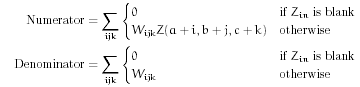
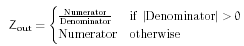
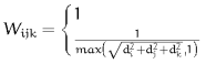
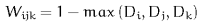
 where Wijk represents the weights defined for the specified filter and
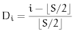
 where
where

 where
where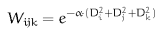 where
where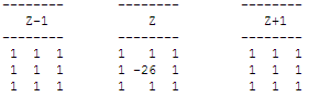
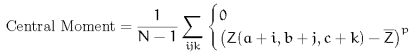
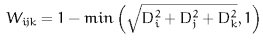
 as shown on the right. Third, compute the local variance as shown on the right.
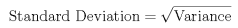
 where
where  represents the mean
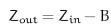 where
where  represents the median
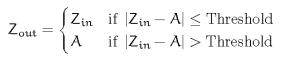
 represents the average value
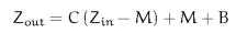
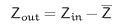
 represents brightness,
  represents contrast, and
  is the global midrange for the entire lattice.