 button to the right of the
Colormap option
in the Property Manager
to open the Colormap Editor dialog.
button to the right of the
Colormap option
in the Property Manager
to open the Colormap Editor dialog.The Colormap Editor dialog is used to create custom colors and effects for use as a Colormap.
Click the button to the right of the
Colormap option
in the Property Manager
to open the Colormap Editor dialog.

Use the Colormap
Editor dialog to create custom
colors for a Colormap.
The Colormap Editor dialog sections are described below.
The upper section of the dialog contains the opacity mapping controls. These controls specify how a range of data values are mapped to opacity in the final output. Note that opacity is the opposite of transparency (0.0 is completely transparent, 1.0 is completely opaque).
The Opacity Mapping drop-down displays a series of predefined opacity settings. These may be used to preset the opacity settings which can then be modified as desired. The Opacity Graph is updated to display the selection.
Choose one of predefined opacity maps:
· Fixed 0.2 sets the entire range of data to a fixed opacity of 0.2.
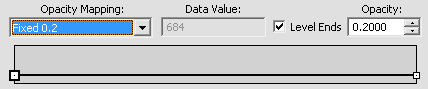
The Opacity Mapping predefined
setting of Fixed 0.2 sets
the
Opacity to a constant 20%.
· Fixed 1.0 sets the entire range of data to a fixed opacity of 1.0 (fully opaque).
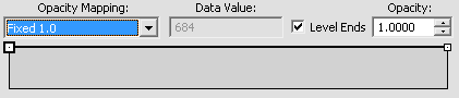
The Opacity Mapping predefined
setting of Fixed 1.0 sets the
Opacity to a constant 100%.
· Ramp 0.0 to 0.2 sets the smallest data values to an opacity of 0.0 and the largest data value to an opacity of 0.2. The opacity of the middle values increases linearly.
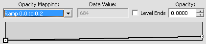
The Opacity Mapping predefined
setting of Ramp 0.0 to 0.2 sets
the
Opacity to go from 0% to 20%.
· Ramp 0.0 to 1.0 sets the smallest data values to an opacity of 0.0 and the largest data value to an opacity of 1.0. The opacity of the middle values increases linearly.
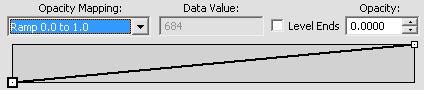
The Opacity Mapping predefined
setting of Ramp 0.0 to 1.0 sets
the
Opacity to go from 0% (fully transparent)
to 100% (fully opaque).
· Middle Ramp sets the lowest quartile to 0.0 opacity, followed by a linear ramp over the middle half of the data, followed by a fixed opacity of 1.0 for the last quartile.
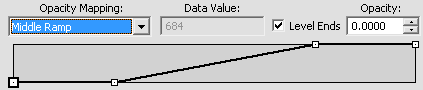
The Opacity Mapping predefined
setting of Middle Ramp sets the
Opacity to go from 0% to 100% in the
middle of the data range.
· Custom is added as an option automatically when a node is selected, created, removed, or the Opacity value or Data Value options are adjusted.
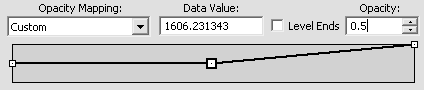
The Opacity Mapping predefined
setting of Custom is
created when any
adjustments are made to one of the Opacity Mapping
predefined settings.
Data Value displays the data value of the node selected in the opacity graph. The selected node may be accurately repositioned by entering a new value here. The first and last nodes cannot be changed and this control is disabled (grayed out) when an end node is selected.
Check the Level Ends box to level the first and last segments of the opacity graph. When the nodes at one end of a level segment are dragged up or down, the other end is also dragged.
Choose the level of opacity. This value ranges from 0.0 (completely
transparent) to 1.0 (completely opaque). To change the opacity, click
on one of the nodes. Then, highlight the existing value and type a new
value or click the  button to increase or decrease the
opacity for the selected node.
button to increase or decrease the
opacity for the selected node.
The graph consists of a background histogram showing the distribution of data values. A series of two or more nodes (represented by white squares) are connected by line segments. The selected node is drawn as a larger square. Each node is a moveable anchor point whose horizontal position represents a data value, and whose vertical position represents the desired opacity at that data value. The opacity for data values between nodes is calculated by linear interpolation.
Here are some notes about the opacity graph:
Left-click a node to select it. A selected node is highlighted with a thick black border.
Use the left and right arrow keys on your keyboard to select the previous or next node.
New nodes may be added by double-clicking the graph at the desired location or by pressing the INSERT key. When INSERT is pressed, a new node is added adjacent to the selected node, half the distance to the next node.
Press the DELETE key to delete the selected node. The end nodes cannot be deleted.
Left-click and drag nodes with the mouse to move them. Nodes cannot be moved past their neighbors. End nodes cannot be moved horizontally. This makes it easier to align two nodes vertically in order to get an abrupt transition.
Nodes can be moved directly atop one another.
The histogram uses the logarithm of the counts in order to display widely disparate data. Using the counts directly results in extreme highs and 0 everywhere else for most data sets.
The middle section of the dialog contains the color mapping controls, which are similar to the opacity mapping controls but affect the colors assigned to the data rather than the opacity.
The color mapping drop-down displays a series of predefined color maps. These may be used to preset the color map which can then be modified as desired.
Data Value displays the data value of the node selected in the color graph. The selected node may be accurately repositioned by entering a new value here. Note that the first and last nodes cannot be changed and this control is disabled when an end node is selected.
Click the  or the
  button to toggle between
setting values for RGB (red, green, blue) and HSL
(hue, saturation, luminance) modes.
button to toggle between
setting values for RGB (red, green, blue) and HSL
(hue, saturation, luminance) modes.
RGB specifies the colors as a combination of red, green, and blue. Each component can range from 0 to 255, e.g., black has an RGB of 0,0,0; white has an RGB of 255,255,255; and red has an RGB of 255,0,0.
HSL mode includes hue, saturation, and light. Each component can range from 0 to 255. Hue represents the dominant wavelength of the color and is often represented as an angle defining the different hues along the circumference of a circle. Saturation indicates how much of the hue is mixed into the color. Luminance is also known as brightness or intensity and represents how much light is in the color.
The three edit boxes to the right allow you to enter the individual color components for the currently selected color node. Alternatively, click on the Color drop-down list to pick a color from a list of examples.
The color graph consists of a background histogram showing the distribution of data values. A series of two or more nodes (represented by colored squares) is connected with line segments. The selected node is drawn with a larger frame around it. Each node is a moveable anchor point whose horizontal position represents a data value and whose color represents the desired color at that data value. The color for data values between nodes is calculated by the interpolation method specified in the Interp list.
Here are some notes about the color graph:
The histogram uses the logarithm of the counts in order to display widely disparate data. Using the counts directly results in extreme highs and 0 everywhere else for most data sets.
Click a node to select it.
Use the left and right arrow keys to select the previous or next node.
New nodes may be added by double-clicking the graph at the desired location or by pressing the INSERT key. When INSERT is pressed, a new node is added adjacent to the selected node.
Press the DELETE key to delete the selected node. Note that end nodes cannot be deleted.
Drag nodes with the mouse to move them. Note that nodes cannot be moved past their neighbors, and that end nodes cannot be moved horizontally. This makes it easier to align two nodes vertically in order to get an abrupt transition.
Since the vertical position of nodes within the color graph is irrelevant, coincident nodes are automatically moved up or down so they do not conflict. Note that this is only done for two coincident nodes. A third coincident node obscures the second (and so on). In this case, clicking repeatedly on the coincident nodes cycles through them, selecting each one in turn.
A sample of the generated Colormap appears directly below the color graph.
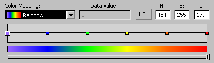
The gradational purple to red Colormap example display appears below
the color graph section with nodes for each color.
The scroll control appears as a three-dimensional horizontal bar with draggable end handles. Drag a handle left or right to zoom the graphs in or out. When zoomed in, the center section becomes blue. Drag the center blue section to scroll the visible portion left or right. Double-click the center section to return it to the fully visible state.
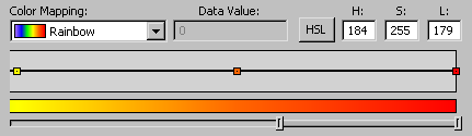
The scroll bar below the Colormap Example allows you to zoom in on
a section of the Colormap. In this example, the scroll bar was dragged
to zoom in on the yellow, orange, and red nodes.
The bottom section of the dialog allows selection of data minimum and maximum values, individual color picks, and how the color map should be interpolated. In addition, you can load or save a colormap or close the dialog.
Colormaps process data with values over a specified range. The Data Min and Data Max values correspond with the left and right edges of the Colormap, respectively. Data outside this range are clipped at the corresponding edge of the Colormap. Clipped data are not displayed. The minimum and maximum fields can be set to any desired value. If you wish to reverse the color map, change the Data Min value so that it is greater than the Data Max value.
Check the Use data limits box to set the Data Min and Data Max values to the limits of the input data. This results in the Colormap mapping the entire range of the input data without any clipping at the ends.
Click the Color box to specify the color of the currently selected node. The color palette opens. Click the More Colors button to open the Colors dialog.
Choose the interpolation method used between nodes in the Colormap.
Linear interpolation uses weighted averages to move over nodes from the first color to the last color. This linear interpolation between each color node results in a nice gradational transition and smooth appearance.

The Linear interpolation
results in a smooth transition between nodes.
Reverse interpolation is linear interpolation in reverse and the colors between the nodes are reversed. The colors are linearly interpolated using weighted averages to move over nodes from the first color to the last color. This reverse linear interpolation between each color node results in a segmented appearance.

The Reverse interpolation results in sharp transitions
between nodes.
Cosine interpolation uses 180 degree segments of the cosine wave. The rate of change of the color is faster than the Linear interpolation. This interpolation results in a smooth appearance.

The Cosine interpolation results in a smooth transition
between nodes.
Flat Start, Flat Middle, and Flat End methods of interpolation fill any gaps between nodes with color.

The FlatStart interpolation results
in sharp transitions between nodes.
Flat Start uses
the first color node (the node on the left).

The FlatMiddle interpolation results in sharp transitions between
nodes.
Flat Middle uses interpolation to determine a color in the middle of the
two nodes.

The FlatEnd
interpolation results in sharp transitions between nodes.
Flat End uses the last color node (the node on the right).
HSL Clockwise, HSL
Counter-clockwise, HSL Shortest, and HSL Longest methods of interpolation are based
on the HSL color wheel. The H (hue), S (saturation), and L (luminance)
values are interpreted linearly from the color wheel.

HSL Clockwise interpolates the HSL color wheel in a clockwise direction.

HSL Counter Clockwise interpolates the HSL color wheel
in a counterclockwise direction.

HSL Shortest interpolation is the shortest distance between
Clockwise and Counter Clockwise.

The HSL Longest interpolation is the longest distance between
Clockwise and Counter Clockwise.
Click the Load button to open the Open dialog. Select any saved Colormap File (*.clr) and click the Open button. The Colormap is loaded.
Click the Save button to save the new Colormap properties. The Save As dialog opens. The dialog defaults to saving the Colormap to the Save as type of Colormap Files (*.clr).
Click the Close button to exit the Colormap Editor dialog and save your changes.
Use the Edit | Undo command to reverse the changes made before the Colormap Editor dialog was opened.
See Also