Gridding Methods

Voxler has several different gridding methods available for the Gridder module. The differences between gridding methods are in the mathematical algorithms used to compute the weights during lattice node interpolation. Each method can result in a different representation of the data. You may want to test each method with a known data set to determine the method that provides you with the most satisfying interpretation of the data.

Gridding methods include:

• Inverse Distance to a Power
• Local Polynomial
• Data Metric

Choosing a Gridding Method

Grid method parameters control the interpolation procedures. When you create a lattice with the Gridder module, accept the default method and parameters for acceptable output in most cases. Different methods provide different interpretations of the data because each method calculates lattice node values using a different algorithm. If you are not satisfied with the graphic output from the lattice, consider different methods and parameters and compare the results.

General Gridding Recommendations

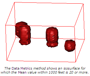
The Data metrics method is used to calculate statistics about a data set.

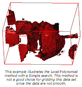
The Local polynomial method is most applicable to data sets that are locally smooth, i.e., relatively smooth surfaces within the search neighborhoods. The computational speed of the method is not significantly affected by the size of the data set.

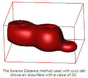
The default Inverse distance method is fast but has the tendency to generate concentric spheres around high and low values unless you increase the Smooth value. This method does not extrapolate beyond the Z range of the data.

Inverse Distance to a Power Gridding Method

The Inverse distance method is a weighted average interpolator and can be either an exact or a smoothing interpolation.

Data are weighted during interpolation such that the influence of a point declines with distance from the lattice node. Weighting is assigned to data using a weighting Power that controls how the weighting factors drop off as distance from a lattice node increases. The greater the power, the less effective points far from the lattice node have during interpolation. As the power increases, the lattice node value approaches the value of the nearest point. For a smaller power, the weights are more evenly distributed among the neighboring data points.

Inverse distance normally behaves as an exact interpolator. When a grid node is calculated, the weights assigned to the data points are fractions, and the sum of all the weights is equal to 1.0. When a particular observation coincides with a lattice node, the distance between that observation and the node is 0.0, and that observation is given a weight of 1.0 while all other observations are given weights of 0.0. Thus, the grid node is assigned the value of the coincidental observation. The Smooth parameter is a mechanism for buffering this behavior. When you assign a non-zero Smooth value, no point is given an overwhelming weight so that no point is given a weighting factor equal to 1.0.

One of the characteristics of inverse distance is the generation of concentric spheres surrounding the position of observations within the lattice. To reduce the effect, assign a Smooth value other than 0.

Inverse Distance to a Power Equations

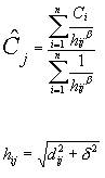
The following equations are used for Inverse Distance to a Power:

where:

is the effective separation distance between grid node " j" and the neighboring point "i";

is the interpolated value for grid node " j";

are the neighboring points;

is the distance between grid node " j" and the neighboring point "i";

is the Power or weighting parameter; and

is the Smooth parameter.

Inverse Distance to a Power References

Davis, John C. (1986) Statistics and Data Analysis in Geology. John Wiley and Sons, New York, NY.

Franke, R. (1982) Scattered Data Interpolation: Test of Some Methods, Mathematics of Computations, v. 33, n. 157, p. 181-200.

Local Polynomial Gridding Method

The Local polynomial method assigns values to lattice nodes by using a weighted least squares fit with data within the search ellipsoid.

For each lattice node, the neighboring data are identified by the user-specified Search type and Count. Using only data that match the search criteria, a local polynomial is fit using weighted least squares; the lattice node value is set equal to this value. Local polynomials can be order 1, 2, or 3.

Data Metric Gridding Method

The Data Metric method is used to calculate statistical values using the data points found within the search. Define the search with the Search Type parameters. These search parameters are applied to each grid node to determine the local data set.

Comparison of Gridding Methods

The following comparison example is using the same data set, gridding with each of the three Method options.

See Also

Introduction to Modules

Data Types

Gridder

Math

Merge

Resample

Slice

Connecting Modules

How do I export a Gridder lattice to ASCII XYZC?

Computational Modules