Gridding Example

In this gridding example, consider the problem of producing isosurfaces of gold concentration given well data collected from boreholes over a region. The well locations are not regularly spaced over the area of interest. Use the File | Import command to load the data into the Network Manager, connect a Gridder module to the data, select the Gridder module in the Network Manager to display the properties in the Property Manager and click the Begin Gridding button to produce a uniform regularly-spaced lattice over the XYZ extents. Add an Isosurface module to the Gridder to display surfaces of equal concentration based on the lattice node values. The steps are detailed below.

Click the File | Import command.
In the Import dialog, select the xyzc1.dat data file, located in the Voxler Samples directory, and click Open.
If the Data Import Options dialog is displayed, select Delimited as the Field Format. Check the Comma box in the Delimiters section. Check the Double Quote box in the Text Qualifiers section and click OK.
In the Property Manager specify the data columns for the X, Y, and Z coordinates and C component.

Set the Output type to Points
Set X coordinates to Column A: X
Set Y coordinates to Column B: Y
Set Z coordinates to Column C: Z
Set Component columns to 1
Set Component-1 to Column D: C

To view the data that was imported, click on the xyzc1.dat module in the Network Manager. In the Property Manager, click the Edit Worksheet button. The linked data is opened in a worksheet document. The document title includes the module name and number. Any changes made to the data while viewing the linked worksheet are automatically saved and applied in the project.
Close the worksheet window, or click on the project file tab, to return to the viewer window.
In the Network Manager, click on the xyzc1.dat module. Click the Network | Graphics Output | ScatterPlot to add a scatter plot to the view. You can change any properties of the ScatterPlot, such as the symbol size and color.
In the Network Manager, click on the xyzc1.dat module. Click the Network | Graphics Output | BoundingBox to add a bounding box to the view.
In the Network Manager, click on the xyzc1.dat module. Click the Network | Graphics Output | Axes to add axes to the view.

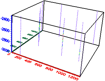
A ScatterPlot of the data set shows the distribution
of the XYZ data points from the borehole sampling.
BoundingBox and Axes modules have also been added.

In the Network Manager, click on the xyzc1.dat module. Click the Network | Computational | Gridder command to attach a Gridder module.
Click on the Gridder module. In the Property Manager, click the Begin Gridding button to start the gridding process using the default options.
In the Network Manager, click on the Gridder module. Click the Network | Graphics Output | Isosurface command to display the gridded data as an Isosurface module. Change any properties of the Isosurface, such as the Isovalue or color.


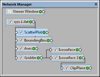
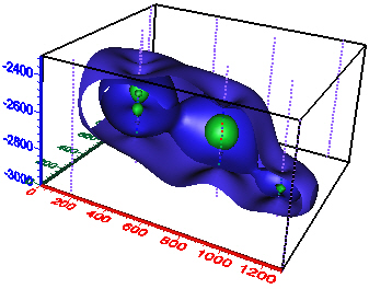
The full network is shown. A ClipPlane module has been added to the isosurfaces to show the interior surfaces.	Isosurfaces have been added to the Gridder module to display surfaces of equal concentration based on the lattice node values.